Detecting Network Intrusions at the Edge
By Dan Howarth
One of the core work packages in the Synergia project is Distributed Intrusion Detection System for the Protection of the Edge, which is focussed on how we can detect network intrusions on resource-constrained edge devices in an IOT network.
The work was led by Smartia, one of the UK’s leading Industrial AI & IOT technology companies. IoT security is a particular focus of Smartia’s research as the adoption of its industrial intelligence platform, MAIO, accelerates.
This blog looks at the machine learning approach we used to detect these network intrusions, and why we chose this approach.
Machine Learning Approach
A machine learning model is typically trained on data that is representative of data it can expect to see when tasked with making predictions. In our case, this is data of the operating system’s activities before, during and after a ‘container escape’ – an event where software that is used to deploy applications – the container – actually hosts a malicious program that breaks out and attacks the edge device.
Our chosen modelling approach would need to meet the following requirements:
- It should be appropriate to the data we were collecting – in particular, the dataset collected by the University of Bristol had a relatively small amount of data for container events compared to data for normal, non-attack conditions;
- It needed to be deployable on an edge device – this means it needed to be fairly small in terms of memory so that it can fit on an edge device and not consume too much power in its execution.
- Finally, it needed to be accurate – we wanted an approach that was powerful and therefore more likely to succeed, as well as something that offered us a lot of flexibility and scope to fine tune and squeeze out as much performance as possible from the model.
Autoencoder
The approach we felt best met these requirements was an autoencoder.
https://commons.wikimedia.org/wiki/File:Autoencoder_schema.png
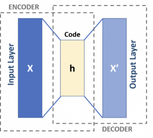
An autoencoder is used to convert a set of data into a smaller representation of itself. It does this by removing noise from the data and focusing on the core dimensions of the data. This encoding can be useful in its own right as a way of compressing large dimensional data into something more manageable for further analysis or modelling activity.
However, we additionally decode this representation using the autoencoder to try and recreate the original data passed to the model. The difference between the original and reconstructed data is captured by a reconstruction error. The lower the reconstruction error, the better able the model is to reconstruct the data.
Figure 1 sets out the high level architecture for an autoencoder.
Semi-supervised Learning
Autoencoders have a variety of uses; in our case, it enabled us to tackle the dataset requirement by adopting a semi-supervised approach – which is designed to deal with situations where there is only a small amount of labelled data.
Our autoencoder is trained on normal (non-event data) only. It is trained until its reconstruction error is very low, so that we are confident that it can reconstruct the encoded normal data passed to it at the decoding stage. When ‘container escape’ data is passed to it, it should return a high reconstruction error – that is, it is unable to effectively reconstruct this data because it is sufficiently different from the normal data.
Flexibility
An autoencoder is a very flexible approach. We are able to implement a wide range of architectures for the encoder and decoder to find the best performance (for example, varying the size and number of layers within the model). And, because it is part of the neural network family of models, it is well supported in machine learning software libraries, making design and implementation straightforward.
Additionally, because of this flexibility and by keeping the architecture small, we are able to design a model that can meet edge deployment constraints.
Results
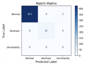
The result of all this approach was a model that was very accurate. Following model training, we tested it on unseen data and applied a threshold to the reconstruction error so that any score above the threshold was classified as an anomaly (attack).
The confusion matrix in Figure 2 shows how well the model performed on the test set. As we can see, it predicted all anomalies correctly and almost all of the normal data too.
This meant an accuracy of over 99%, which is the final piece of evidence that the approach we took was able to meet our requirements.